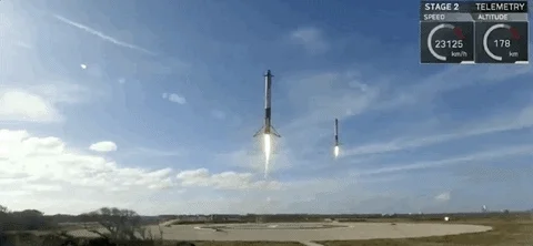
Soft Landing Optimal Control using Convex Optimization

Convex Optimization (MA60213) Autumn 2024 Term Project

Sampreeth R S (21CS30038) & Prasanna Paithankar (21CS30065)

Report PDF

Overview

Soft landing constitutes the concluding step of a planetary EDL (entry, descent, and landing) and is also known as the powered descent landing stage. During the powered descent phase, the ship is manoeuvred as near as feasible to a designated site on the planet’s surface via thrusters that offer control authority. When the vehicle “soft lands,” or lands with zero velocity in relation to the surface, this phase comes to an end. Under thrust and state limitations, our goal is to create a fuel-optimal thrust profile as a function of time that gets the vehicle to its intended destination.

The control restrictions in the original version of the soft-landing powered-descent guiding issue make it a nonconvex finite horizon optimal control problem. The guiding algorithm must provide legitimate thrust vectors with a nonzero minimum and maximum on the thrust magnitude since the descent thrusters cannot be throttled off after initiation. This is a non-convex constraint on the control input. Another cause of nonconvexity is the fact that onboard sensors for terrain-relative navigation often call for particular viewing orientations, which limit the permitted spacecraft orientations and, consequently, the thrust vector pointing direction.

Finding a convex relaxation of the original optimum control issue and demonstrating that an optimal solution to the relaxed problem is likewise optimal for the original problem are the main objectives.

Non-convex problems can be convexified in 2 ways:

Restrict the set of feasible solutions to a convex subset of the feasible set.
Relax the set of feasible solutions to a convex set containing the original set of feasible solutions.

We follow the second method to covexify our problem and prove that the relaxed problem achieves the same optimal value as the original problem.

Objective

We present 2 objectives in this project:

Minimize fuel consumption: \[ \min_{t_f, T_c(\cdot)} \int_0^{t_f} \| T_c(t) \| \, dt. \]

Minimize the landing error: \[ \min_{t_f, T_c(\cdot)} \| E r(t_f) - q \|, \] where \(r(t)\) is the position vector, \(q\) is the desired landing altitude, and \(E\) is a selection matrix.

Physical Dynamics

The lander dynamics are modeled using a lumped mass rigid body with thrust vector for control. The equations governing the dynamics are:

\[ \begin{aligned} \dot{x}(t) = A(\omega) x(t) + B(g + \frac{T_c(t)}{m}) \\ \dot{m}(t) = -\alpha \| T_c(t) \| \end{aligned} \]

where \(x(t) = [r(t), \dot{r}(t)]\) is the state vector \(\in \mathcal{R}^3 \times \mathcal{R}^3\), \(r(t)\) is the position vector, \(\dot{r}(t)\) is the velocity vector, \(m(t)\) is the mass, \(\omega\) is the orientation, \(A(\omega)\) is the rotation matrix, \(B\) is the control matrix, \(g\) is the gravity vector, and \(\alpha\) is the fuel consumption rate.

The matrix \(A(\omega)\) and \(B\) is given by

\[ \begin{aligned} A(\omega) &= \begin{bmatrix} 0 & I \\ -S(\omega)^2 & -2S(\omega) \end{bmatrix} \\ B &= \begin{bmatrix} 0 \\ I \end{bmatrix} \end{aligned} \]

\(\omega = [\omega_1, \omega_2, \omega_3] \in \mathcal{R}^3\) is the planet’s angular velocity and \(S(\omega)\) is the skew-symmetric matrix of \(\omega\).

\[ S(\omega) = \begin{bmatrix} 0 & -\omega_3 & \omega_2 \\ \omega_3 & 0 & -\omega_1 \\ -\omega_2 & \omega_1 & 0 \end{bmatrix} \]

Lumped mass assumption means that translational and rotational dynamics are decoupled. This allows altitude control to be made quickly to maintain the desired thrust direction.

Constraints

The planetary soft landing problem involves constraints on the state and control input. The main constraints are:

Glide Slope Constraint \[ \| E(r(t) - r(t_f)) \| - c^T (r(t) - r(t_f)) \leq 0, \quad \forall t \in [0, t_f] \] where \(E = [e_2^T, e_3^T]^T\) extracts position components, and \(c\) defines the cone’s geometry.
Velocity Constraint \[ \| \dot{r}(t) \| \leq V_{\max}, \quad \forall t \in [0, t_f] \]
Convex upper bound on the thrust magnitude \[ \| T_c(t) \| \leq T_{\max}, \quad \forall t \in [0, t_f] \]
Non-convex lower bound on the thrust magnitude \[ \| T_c(t) \| \geq T_{\min} > 0, \quad \forall t \in [0, t_f] \]
Thrust pointing constraint \[ T_c(t) \cdot \mathbf{n} \geq \cos\theta\, \| T_c(t) \|, \quad \forall t \in [0, t_f] \quad \text{and} \quad \theta \in [0, \pi] \] where \(\mathbf{n}\) is the direction unit vector and \(\theta\) is the maximum deviation angle. When \(\theta \leq 90^\circ\), the constraint is convex.

The Optimization Problem (Non-Convex)

The original non-convex optimization problem is stated as follows:

Minimum Landing Error Problem

\[ \begin{aligned} \min_{\mathbf{T}(\cdot), t_f} & \quad \| Er(t_f) - q \|\\ \text{s.t.} & \quad \dot{x}(t) = A(\omega) x(t) + B(g + \frac{T_c(t)}{m}) \\ & \quad \dot{m}(t) = -\alpha \|T_c(t)\| \\ & \quad x(0) = x_0, \quad m(0) = m_0 \\ & \quad x(t_f) = x_f, \quad m(t_f) = m_f \\ & \quad \| T_c(t) \| \leq T_{\max}, \quad \forall t \in [0, t_f] \\ & \quad \| T_c(t) \| \geq T_{\min} > 0, \quad \forall t \in [0, t_f] \\ & \quad T_c(t) \cdot \mathbf{n} \geq \cos\theta\, \| T_c(t) \|, \quad \forall t \in [0, t_f] \quad \text{and} \quad \theta \in [0, \pi]\\ & r(0) = r_0, \quad \dot{r}(0) = \dot{r}_0\\ & e_1^T r(t_f) = 0, \quad \dot{r}(t_f) = 0 \end{aligned} \]

Minimum Fuel Problem

\[ \begin{equation} \min_{t_f, T_c(\cdot)} \int_0^{t_f} \alpha \| T_c(t) \| \, dt, \end{equation} \] subject to: \[ \begin{align} \| E r(t_f) - q \| &\leq \| d^*_P - q \|, \end{align} \]

where \(d^*_P\) is the closest point on the glide slope to the desired landing point.

Convex Relaxation and Convex Problem Formulation

Convex Relaxation Derivation

We introduce a convex relaxation of these constraints, while guaranteeing that the relaxed problem remains equivalent to the original problem under certain conditions (lossless convexification).

Relaxation of Thrust Constraints

The original control constraints on the thrust magnitude are: \[ \rho_1 \leq \| T_c(t) \| \leq \rho_2, \quad \forall t \in [0, t_f]. \] To convexify this constraint, we introduce a slack variable \(\sigma(t)\) such that: \[ \| T_c(t) \| \leq \sigma(t), \quad \rho_1 \leq \sigma(t) \leq \rho_2. \] The slack variable ensures that the feasible set is convex. However, for the relaxed problem to yield an equivalent solution to the original nonconvex problem, the optimal solution must satisfy \(\| T_c(t) \| = \sigma(t)\) almost everywhere.

Relaxation of Thrust Pointing Constraint

The original nonconvex constraint on the thrust direction is: \[ \hat{n}^T \frac{T_c(t)}{\| T_c(t) \|} \geq \cos \theta, \quad \forall t \in [0, t_f]. \] By introducing the slack variable \(\sigma(t)\) as defined above, this constraint becomes: \[ \hat{n}^T T_c(t) \geq \sigma(t) \cos \theta, \quad \forall t \in [0, t_f], \] which is convex in the variables \(T_c(t)\) and \(\sigma(t)\).

Modified System Dynamics

The dynamics of the system are also modified to accommodate the slack variable. The original mass consumption dynamics are given by: \[ \dot{m}(t) = -\alpha \| T_c(t) \|. \]

In the relaxed problem, this becomes: \[ \dot{m}(t) = -\alpha \sigma(t). \]

Formulation of the Relaxed Convex Optimal Control Problems

With these relaxations, we can now formulate the relaxed convex problems.

Convex Relaxed Minimum Landing Error Problem \[ \min_{t_f, T_c(\cdot), \sigma(\cdot)} \| E r(t_f) - q \|, \] subject to: \[ \begin{align} \dot{x}(t) &= A(\omega)x(t) + B \left( g + \frac{T_c(t)}{m(t)} \right), \\ \dot{m}(t) &= -\alpha \sigma(t), \quad t \in [0, t_f], \\ x(t) &in X, \quad \forall t \in [0, t_f], \\ \| T_c(t) \| &\leq \sigma(t), \quad \rho_1 \leq \sigma(t) \leq \rho_2, \\ \hat{n}^T T_c(t) &\geq \sigma(t) \cos \theta, \\ m(0) &= m_0, \quad m(t_f) \geq m_0 - m_f > 0, \\ r(0) &= r_0, \quad \dot{r}(0) = \dot{r}_0, \\ e_1^T r(t_f) &= 0, \quad \dot{r}(t_f) = 0. \end{align} \]

Convex Relaxed Minimum Fuel Problem \[ \min_{t_f, T_c(\cdot), \sigma(\cdot)} \int_0^{t_f} \alpha \sigma(t) \, dt, \] subject to: \[ \begin{align} \dot{x}(t) &= A(\omega)x(t) + B \left( g + \frac{T_c(t)}{m(t)} \right), \\ \dot{m}(t) &= -\alpha \sigma(t), \quad t \in [0, t_f], \\ x(t) &in X, \quad \forall t \in [0, t_f], \\ \| T_c(t) \| &\leq \sigma(t), \quad \rho_1 \leq \sigma(t) \leq \rho_2, \\ \hat{n}^T T_c(t) &\geq \sigma(t) \cos \theta, \\ m(0) &= m_0, \quad m(t_f) \geq m_0 - m_f > 0, \\ r(0) &= r_0, \quad \dot{r}(0) = \dot{r}_0, \\ e_1^T r(t_f) &= 0, \quad \dot{r}(t_f) = 0, \\ \| E r(t_f) - q \| &\leq \| d^*_P - q \|. \end{align} \]

The convex relaxation guarantees that the optimal solution to these problems coincides with the solution to the original nonconvex problems under certain conditions, thereby enabling efficient computation using convex optimization techniques.

Change of Variables and Convex Approximation

One of the primary sources of nonconvexity in the original problem formulation arises from the dynamics of the spacecraft, specifically the term involving the thrust-to-mass ratio \(\frac{T_c(t)}{m(t)}\). This term appears in the state dynamics as: \[ \dot{x}(t) = A(\omega) x(t) + B \left( g + \frac{T_c(t)}{m(t)} \right), \] where \(m(t)\) is the time-varying mass of the spacecraft, making the dynamics nonlinear and nonconvex.

To address this issue, we introduce a change of variables that linearizes the dynamics while maintaining the feasibility of the solution. The following transformations are applied: \[ \begin{align} \sigma(t) &= \frac{\| T_c(t) \|}{m(t)}, \\ u(t) &= \frac{T_c(t)}{m(t)}, \\ z(t) &= \ln(m(t)). \end{align} \]

Transformed Dynamics

With this change of variables, the mass depletion dynamics are reformulated as: \[ \dot{z}(t) = \frac{\dot{m}(t)}{m(t)} = -\alpha \sigma(t), \] where \(\alpha > 0\) is the fuel consumption rate constant. The state dynamics now become: \[ \dot{x}(t) = A(\omega)x(t) + B \left( g + u(t) \right). \] This transformation removes the nonlinearity in the term \(\frac{T_c(t)}{m(t)}\), resulting in linear state dynamics with respect to the new control variable \(u(t)\).

Convex Constraints

In the transformed variables, the original nonconvex constraints on thrust magnitude are replaced with convex constraints on \(\sigma(t)\) and \(u(t)\). Specifically, the constraints become: \[ \begin{align} \| u(t) \| &\leq \sigma(t), \\ \rho_1 e^{-z(t)} &\leq \sigma(t) \leq \rho_2 e^{-z(t)}, \end{align} \] where \(\rho_1\) and \(\rho_2\) are the minimum and maximum thrust magnitudes, respectively.

To ensure a convex formulation, we approximate the bounds on \(\sigma(t)\) using a second-order cone (SOC) constraint: \[ \rho_1 e^{-z_0} \left( 1 - (z(t) - z_0) + \frac{(z(t) - z_0)^2}{2} \right) \leq \sigma(t) \leq \rho_2 e^{-z_0} \left( 1 - (z(t) - z_0) \right), \] where \(z_0(t) = \ln(m_0 - \alpha \rho_2 t)\) is an estimate of the mass trajectory. This approximation ensures that the constraints on \(\sigma(t)\) remain convex and compatible with the overall convex optimization framework.

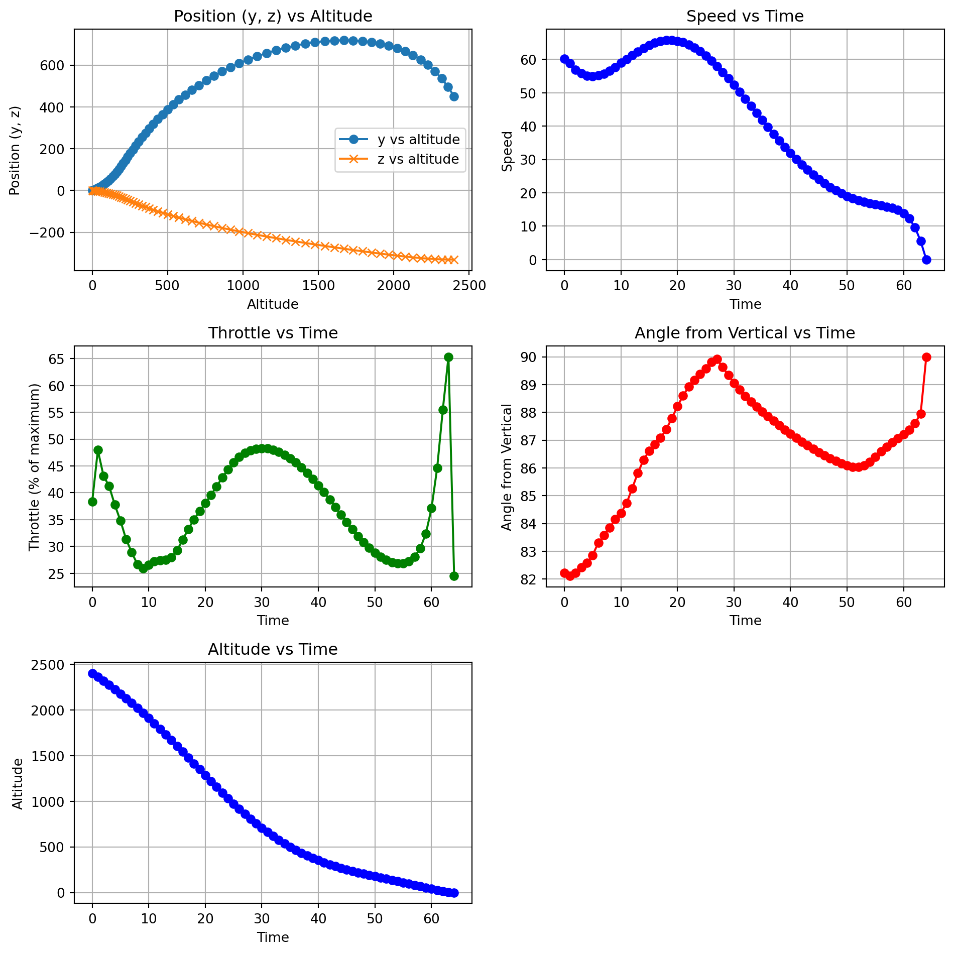
Sample Solution

We solve the convex relaxation of the problem using cvx library in C++ and use discretization over a finite horizon using Interior Point Methods (IPM). We output optimal path and control inputs for the lander.

The following table presents the initial state and attributes of the sample problem:

Parameter	Value	Description
\(m_0\)	2000 kg	Initial mass
\(m_f\)	300 kg	Final mass
\(T_{\min}\)	0.2 \(T_{\max}\)	Minimum thrust
\(T_{\max}\)	24000 N	Maximum thrust
\(\alpha\)	5 x 10^-4 s/m	Fuel consumption rate
\(r_0\)	(2400, 450, -330) m	Initial position
\(\dot{r}_0\)	(-40, 45, 0) m/s	Initial velocity
\(g\)	(-3.71, 0, 0) m/s^2	Gravity vector
\(\omega\)	(2.53 x 10^-5, 0, 6.62 x 10^-5) rad/s	Angular velocity
\(q\)	0 m	Desired landing altitude

Define the constants and run the solver

// Include the necessary libraries

double T_max = 24000;

lander_solve::lander_solve_lander_data lander_data = {
        .m_0 = 2000,
        .m_f = 300,
        .rho_1 = 0.2 * T_max,
        .rho_2 = 0.8 * T_max,
        .alpha = 5e-4,
        .V_max = 90
};

lander_solve::lander_solve_trajectory_data trajectory_data = {
        .r_0 = {2400, 450, -330},
        .r_dot_0 = {-40, 45, 0},
        .gamma_gs = M_PI / 6,
        .theta = 2 * M_PI / 3,
        .n_hat = {1, 0, 0},
        .q = {0, 0}
};

lander_solve::lander_solve_planet_data planet_data = {
        .g = {-3.71, 0, 0},
        .omega = {2.53e-5, 0.0, 6.62e-5}
};

After defining the constants, we run the solver to get the optimal path and control inputs.

lander_solve::lander_solve lander_solve{lander_data, trajectory_data, planet_data, 65, 105, 1, dt};

if (!lander_solve.compute()) {
    std::cout << "Infeasible" << std::endl;
    return 1;
}

Plot the optimal path and control inputs

import pandas as pd
import matplotlib.pyplot as plt

data = pd.read_csv('./Assets/trajectory_output.csv')

data.columns = ['time', 'x', 'y', 'z', 'vx', 'vy', 'vz', 'throttle', 'angle_from_vertical', 'speed']

fig, axs = plt.subplots(3, 2, figsize=(10, 10))

# Plotting position (y, z) with respect to x
axs[0, 0].plot(data['x'], data['y'], label='y vs altitude', marker='o')
axs[0, 0].plot(data['x'], data['z'], label='z vs altitude', marker='x')
axs[0, 0].set_xlabel('Altitude')
axs[0, 0].set_ylabel('Position (y, z)')
axs[0, 0].set_title('Position (y, z) vs Altitude')
axs[0, 0].legend()
axs[0, 0].grid(True)

# Plotting speed with respect to time
axs[0, 1].plot(data['time'], data['speed'], label='Speed', color='b', marker='o')
axs[0, 1].set_xlabel('Time')
axs[0, 1].set_ylabel('Speed')
axs[0, 1].set_title('Speed vs Time')
axs[0, 1].grid(True)

# Plotting throttle with respect to time
axs[1, 0].plot(data['time'], data['throttle'], label='Throttle', color='g', marker='o')
axs[1, 0].set_xlabel('Time')
axs[1, 0].set_ylabel('Throttle (% of maximum)')
axs[1, 0].set_title('Throttle vs Time')
axs[1, 0].grid(True)

# Plotting angle from vertical with respect to time
axs[1, 1].plot(data['time'], data['angle_from_vertical'], label='Angle from Vertical', color='r', marker='o')
axs[1, 1].set_xlabel('Time')
axs[1, 1].set_ylabel('Angle from Vertical')
axs[1, 1].set_title('Angle from Vertical vs Time')
axs[1, 1].grid(True)

# Plotting altitude with time
axs[2, 0].plot(data['time'], data['x'], label='Altitude', color='b', marker='o')
axs[2, 0].set_xlabel('Time')
axs[2, 0].set_ylabel('Altitude')
axs[2, 0].set_title('Altitude vs Time')
axs[2, 0].grid(True)

# Hide the empty subplot
fig.delaxes(axs[2, 1])

plt.tight_layout()
plt.show()

The Optimal Trajectory

import plotly.express as px
import pandas as pd

data = pd.read_csv('./Assets/trajectory_output.csv')

fig = px.scatter_3d(data, x='z', y='y', z='x', color='time')
fig.show()

Equivalence Between Convex Relaxation and Original Nonconvex Problem

We prove that the convex relaxation described earlier produces the same optimal solution as the original nonconvex problem under specific conditions. This result is often referred to as a lossless convexification, meaning that the solution of the relaxed problem is guaranteed to satisfy the constraints of the original problem while achieving the same optimal value.

Theoretical Background and Lemma

The convex relaxation is based on relaxing the nonconvex constraints on thrust magnitude and pointing direction by introducing a slack variable \(\sigma(t)\). We denote the set of feasible solutions for the original nonconvex problem by \(F\) and for the relaxed convex problem by \(F_{\text{convex}}\). The relaxation is considered lossless if:

\[ \| \mathbf{T}^*(t) \| = \sigma^*(t) \text{ a.e. on } [0, t_f] \]

where \((\mathbf{T}^*(t), \sigma^*(t))\) is an optimal solution of the convex problem.

Lemma

Given an optimal solution \((\mathbf{T}^*(t), \sigma^*(t)) \in F_{\text{convex}}\) such that \(\| \mathbf{T}^*(t) \| = \sigma^*(t)\) almost everywhere on \([0, t_f]\), the solution \(\mathbf{T}^*(t)\) also belongs to the feasible set of the original nonconvex problem \(F\).

Proof. Consider the relaxed constraints:

\[ \begin{aligned} \| \mathbf{T}^*(t) \| &\leq \sigma(t), \quad \rho_1 \leq \sigma(t) \leq \rho_2 \\ \mathbf{n}^T \mathbf{T}^*(t) &\geq \sigma(t) \cos \theta \end{aligned} \]

Let \((\mathbf{T}^*(t), \sigma^*(t))\) be an optimal solution to the relaxed problem. By construction, the slack variable \(\sigma(t)\) is introduced to ensure convexity while maintaining a feasible set that contains the feasible region of the original problem. We need to show that:

\[ \| \mathbf{T}^*(t) \| = \sigma^*(t) \text{ a.e. on } [0, t_f] \]

Since the cost function is minimized with respect to \(\| \mathbf{T}^*(t) \|\) (e.g., total fuel consumption), achieving equality \(\| \mathbf{T}^*(t) \| = \sigma^*(t)\) provides the minimum cost for the relaxed problem. If \(\| \mathbf{T}^*(t) \| < \sigma^*(t)\) for any measurable subset of \([0, t_f]\) with positive measure, reducing \(\sigma^*(t)\) to match \(\| \mathbf{T}^*(t) \|\) would strictly decrease the cost, contradicting the optimality of \((\mathbf{T}^*(t), \sigma^*(t))\).

Thus, the condition \(\| \mathbf{T}^*(t), \sigma^*(t)\) holds almost everywhere, implying that the solution \(\mathbf{T}^*(t)\) satisfies the original thrust magnitude constraints:

\[ \rho_1 \leq \| \mathbf{T}^*(t) \| \leq \rho_2 \]

Furthermore, the thrust pointing constraint in the relaxed problem:

\[ \mathbf{n}^T \mathbf{T}^*(t) \geq \sigma(t) \cos \theta \]

combined with the condition \(\| \mathbf{T}^*(t) \| = \sigma^*(t)\), ensures that:

\[ \mathbf{n}^T \mathbf{T}^*(t) \geq \cos \theta \]

This satisfies the original nonconvex thrust pointing constraint.

Therefore, the optimal solution \(\mathbf{T}^*(t)\) for the relaxed problem is also an optimal solution for the original nonconvex problem.

Thank you!

Term Project for the course Convex Optimization (MA60213) at IIT Kharagpur, Autumn 2024.

References

[1] B. A¸cıkme¸se, J. M. Carson III, and L. Blackmore, “Lossless Convexification of Nonconvex Control Bound and Pointing Constraints of the Soft Landing Optimal Control Problem.”

[2] B. A¸cıkme¸se and S. R. Ploen, “Convex programming approach to powered descent guidance for Mars landing,”” Amer. Inst. Astron. Aeron. J. Guid., Control Dyn., vol. 30, no. 5, pp. 1353–1366, 2007.