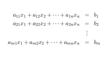
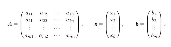
Consider a system of m linear equations in n variables:
Two dimensional arrays are widely used to represent matrices. Let us plan for matrices as big as 20x20 and have a (static) two-dimensional array for storing the elements. We also need the exact number of rows and columns in a matrix.
#define MAX_DIMEN 20
typedef struct {
   int rowdim;                              /* Number of rows */
   int coldim;                              /* Number of columns */
   float element[MAX_DIMEN][MAX_DIMEN];     /* The elements */
} matrix;
Since we are dealing with square system of equations only, we
will always have the equality of row and column dimensions in
our square matrices. In that case holding a single dimension
in the matrix structure would be sufficient. But for the sake
of generality let us allow the possibility of treatment of
mxn matrix.
A vector, on the other hand, can be represented by a one-dimensional array as follows:
typedef struct {
   int dim;                                 /* Dimension of a vector */
   float element[MAX_DIMEN];                /* The elements */
} vector;
Compute the inverse A-1 of A (provided that A is non-singular, i.e., invertible). You can use the following algorithm for this computation:
By an elementary row operation on a matrix we mean one of the following operations (Note that each row corresponds to an equation.):
Start with A and another matrix B. Assume that A is an nxn matrix. B should be initialized to the nxn identity matrix I (the matrix with 1 in its main diagonal and zero elsewhere). Use a sequence of elementary row operations on A to convert it to the identity matrix. Apply the identical sequence of elementary row operations on B. When A is reduced to I, B is transformed to the inverse of A. If A can not be reduced to I, A is not invertible; report `failure' in this case.
The reduction of A to I consists of n iterative steps indexed by i=1,...,n. At the beginning of the i-th iterative step the first through (i-1)-th columns have been converted to the first i-1 columns of I. During the i-th iterative step we reduce the i-th column of A to the i-th column of I using elementary row operations. The ii-th entry of I is one. So we search for a non-zero entry among aki, k=i,...,n. If no such entry is found, report failure and terminate. If aii=0 and aki!=0 for some k>i, then interchange row i and row k. This brings a non-zero entry at the (new) ii-th location. Now divide the i-th row by the entry aii, so that we now obtain aii=1. When this is done, we make aki=0 for each k!=i by subtracting an appropriate multiple of the i-th row from the k-th one.
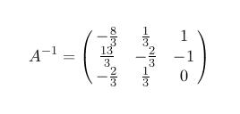
The following figure demonstrates a successful computation of the inverse of a matrix (Here Ri denotes the i-th row.):
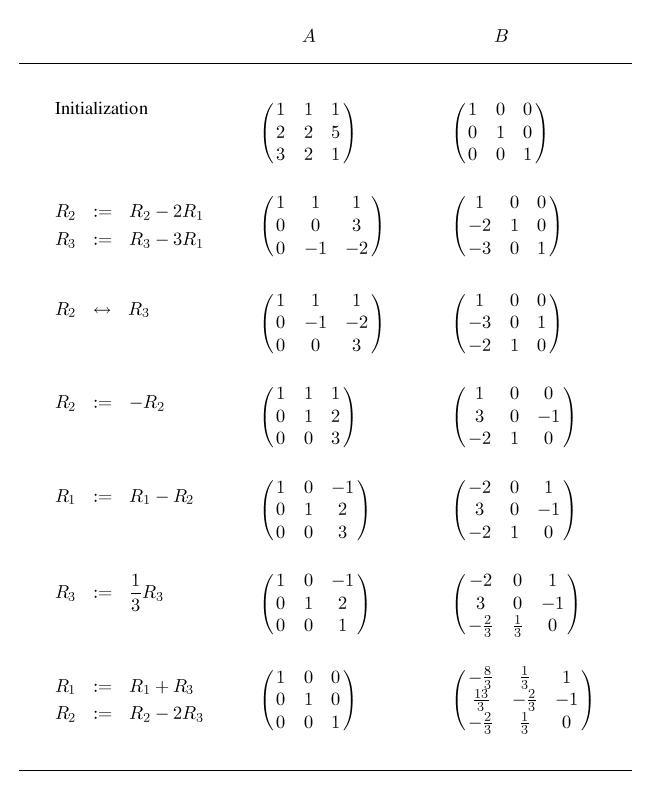
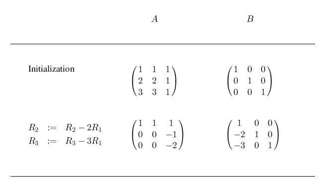
This algorithm computes A-1 in B at the end of the n-step iterative process, provided that A is invertible. On the other hand, if A is not invertible, this algorithm detects it at some stage and reports `failure'. Ask your maths teacher why this algorithm always woks as claimed.
Finally note that in C indexing of arrays starts from zero, whereas we have started numbering of equations and variables from 1. Do the relevant changes in the 1-based indexing scheme in the above description to convert it to the 0-based scheme suitable for C.
Using the value of A-1 computed as above solve the system as:
x = A-1b
Now use your solution x to compute Ax and verify that this x satisfies Ax=b (within floating point approximations).
A sample output is given below:
A :
 -5.00000   0.00000  -4.00000  -8.00000   9.00000   6.00000   7.00000  -7.00000
  6.00000   8.00000 -10.00000  -7.00000  10.00000   9.00000  -3.00000  -5.00000
  3.00000  -1.00000  10.00000  -4.00000   7.00000 -10.00000   8.00000   1.00000
  2.00000   2.00000  -7.00000   5.00000   6.00000   2.00000   9.00000 -10.00000
 -8.00000  -8.00000  -8.00000 -10.00000   8.00000   8.00000  -9.00000   2.00000
  5.00000  10.00000   5.00000   2.00000   9.00000  10.00000   7.00000   1.00000
 -2.00000   5.00000   7.00000  -6.00000   3.00000   2.00000   4.00000  -6.00000
 -6.00000   5.00000  10.00000   8.00000  -3.00000   6.00000   8.00000  -1.00000
b :
  9.00000   9.00000  -3.00000   4.00000   4.00000  -4.00000  -5.00000  -2.00000
Inverse of A :
 -0.01828  -0.26724  -0.16397   0.07274  -0.01426   0.23921   0.18380  -0.31933
  0.01915   0.33907   0.16668  -0.11296  -0.05370  -0.23245  -0.19760   0.31257
 -0.08421  -0.13234  -0.04793   0.05484   0.04918   0.10096   0.15943  -0.10244
 -0.10606   0.05603   0.05134   0.06916   0.05217  -0.04345  -0.03610   0.09941
 -0.08829   0.12891   0.12760   0.04010   0.07738  -0.07417  -0.05894   0.13431
  0.01840  -0.22616  -0.16725   0.04163   0.01591   0.20245   0.14410  -0.21178
  0.15023  -0.07223  -0.03655  -0.04358  -0.07914   0.05678  -0.05564  -0.05885
  0.09201   0.10213   0.06998  -0.11869  -0.04355  -0.04395  -0.18903   0.10532
x :
 -3.08096   3.35002  -2.38514   0.03657   0.77546  -2.24474   0.48955   1.79862
Original b :
  9.00000   9.00000  -3.00000   4.00000   4.00000  -4.00000  -5.00000  -2.00000
Reconstructed b :
  9.00000   9.00002  -3.00000   4.00000   3.99998  -3.99999  -5.00000  -2.00001
Look at the effect of floating point approximations. The reconstructed b is slightly different from the original b. These floating point errors can be reduced by a technique called pivoting. Interested students can look at books on numerical analysis to know more about this.
Remark: We recommend you to implement the following functions:
[Course home] [Home]