Partha Bhowmick: Random Curve Generation

Random Curve Generation

(A linear-time algorithm with artistic emulation)

Algorithm
Partha Bhowmick and Reinhard Klette, Generation of Random Digital Simple Curves with Artistic Emulation, Journal of Mathematical Imaging and Vision, Springer, Vol. 48(1), pp. 53-71, 2014.

Background: The problem of generating random curves is quite interesting, whose historical origin can be traced back to several classical studies on Brownian motion and random walk. Closed random curves also find a resemblance with polygons whose generation has received considerable attention in recent times.

There is no published work till date on generating (closed and irreducible) random digital curves. A polygon-generation algorithm works with vertices of the polygon as input, generated randomly but a priori. On the contrary, our algorithm generates the points on the fly while creating the digital curve C. Starting from a random point (vertex) p₁, it choose the next safe point p₂ randomly, connects the points p₁ and p₂, again chooses the next safe point p₃ randomly and connects it with p₂, and so forth, and eventually ends at the start point p₁, thereby generating a closed digital curve.

Applications: For testing an algorithm A that takes a digital curve as input. Ideally, one would like to test the behavior and performance of A on various real-world digital curves, which are often very difficult to obtain. So a proven algorithm is necessary to generate a sufficiently large set of random curves of finite length in the digital plane.

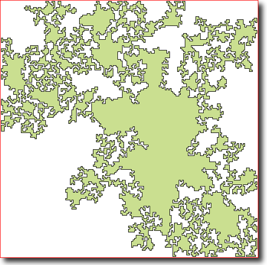
Artistic emulation: A curve-constrained domain is defined by the Minkowski sum of the input drawing with a structuring element whose size varies with the pencil diameter. An artist's usual trait of making irregular strokes and sub-strokes, with varying shades while sketching, is thus captured in a realistic manner. Algorithmic solutions of non-photorealism are perceived as an enrichment of contemporary digital art.

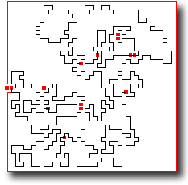
Problem difficulty lies in generating a curve C on the fly such that C never intersects or touches itself, and hence becomes simple and irreducible. This, in turn, calls for detecting every possible narrow-mouthed trap formed by a previously generated part of C, which, if entered into, cannot be exited without touching or intersecting C.

Detecting and avoiding a trap: A trap may be arbitrarily nested in multiple and has to be detected fast without any backtracking (due to some already-entered part of the curve through the mouth of the trap) in order to minimize the computations involved. Further, since C has to be closed, it must be ensured that the (k-connected) path traced by the algorithm finally reaches the very start point.

Proof of correctness: Follows from the principle of mathematical induction.

Runtime: Linear in the length of C.

Theoretical Foundation

Some important theorems are given below. For other theoretical results, see the paper.

Theorem 1	There exists a free path from the current cell $c_i$ to the start cell $c_1$ if and only if $A_1(c_i)\cap R_i\neq\emptyset$. Note: A point in the digital plane $\mathbb Z^2$ is said to be a digital point. The set of four horizontally and vertically adjacent points of a point $p(x,y)$ is called the 4-neighborhood (4-N) of $p$, given by: $N_4(p)=\{(x',y'): \|x-x'\|+\|y-y'\|=1\}$. Similarly, the 8-neighborhood (8-N) of $p$ is: $N_8(p)=\{(x',y'): \max(\|x-x'\|,\|y-y'\|)=1\}$. Each point in $N_k (k=4 \mbox{ or } 8)$ is said to be a $k$-neighbor of $p$. The (cellular) open region $R_i$ corresponding to the current cell $c_i$ is the maximal set of free cells of the canvas such that there exists a free path from each cell of $R_i$ to the free border cell (i.e., $c_1^{(5)}$).
Ensuing hole	$E_i\subset R_i$ is an ensuing hole corresponding to $c_i$ if and only if: e1) there exists $c\in {\tilde{N}}(c_i)$ such that $\delta(c, i)=\mathtt{B}$, e2) for each $c'\in E_i$, we have that $\delta(c', i)\in\{\mathtt{L},\mathtt{R},\mathtt{X}\}$, e3) there exists a free path $\rho\left(c_{i+1},c_1^{(5)}\right)$, and for any such path, $c$ is on $\rho\left(c_{i+1},c_1^{(5)}\right)$. Note: Only the cells belonging to the region ${\tilde{N}}(c_i)=A_0(c_i)\smallsetminus(A_1(c_{i-1})\cup A_1(c_{i+1}))$ are labelled in the $i$th iteration.
Corollary1	The edge between $c_i$ and $c_i^{(t)}$ is safe if and only if $c_i^{(t)}$ belongs to $R_i$.
Theorem 2	When the construction of $\rho$ is over, each cell $c$ can have either $\beta(c)\geq16$ ($c$ is occupied) or $\delta(c)\in\{\mathtt{L},\mathtt{R},\mathtt{X}\}$; that is, $\mathtt{B}$ can be the interim label but cannot be the final label of any free cell.
Corollary2	Either a hole or an ensuing hole is created if and only if at least one free cell in ${\tilde{N}}(c_i)$ gets the label $\mathtt{B}$ as $c_i$ becomes the current cell.
Theorem 3	The current cell $c_i$ gives rise to an ensuing hole $E_i$ if and only if there exists a free cell $b_i\in {\tilde{N}}(c_i)$ such that: E1) $\delta(b_i, i)=\mathtt{B}$; E2) $\exists\ \rho(a_i,b_i)\subseteq A_0(c_{i+1})$ for each $a_i\in E_i\cap A_1(c_{i+1})$.
Corollary3	$c_i$ gives rise to a hole $H_i$ if and only if E1 is true and E2 is false.